See the code on GitHub

MNIST from Scratch

This is a blog detailing how to achieve 94% correctness in MNIST using only Numpy. We start with establishing a PyTorch based model as a benchmark, then we implement the same model without PyTorch. We derive equations to update the weights of a two layer fully connected model and implement them with Numpy. Initially, my manual implementation underperforms the benchmark, this is found to be caused by saturation from poor weight initialisation. After correcting this, equivalent performance is achieved and some further analysis is offered.

Background

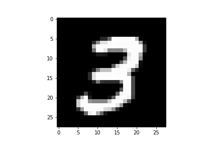
MNIST is a classic image classification dataset consisting of 60k 28 x 28 grayscale images of handwritten numbers and corresponding labels.

Benchmark

I asked ChatGPT to solve MNIST with PyTorch, it gave me a very effective model:

class CNN(nn.Module):
    def __init__(self):
        super(CNN, self).__init__()
        self.conv1 = nn.Conv2d(1, 32, kernel_size=3, padding=1)
        self.conv2 = nn.Conv2d(32, 64, kernel_size=3, padding=1)
        self.pool = nn.MaxPool2d(2, 2)
        self.fc1 = nn.Linear(64 * 7 * 7, 128)
        self.fc2 = nn.Linear(128, 10)
        self.relu = nn.ReLU()
        self.softmax = nn.Softmax(dim=1)

    def forward(self, x):
        x = self.pool(self.relu(self.conv1(x)))
        x = self.pool(self.relu(self.conv2(x)))
        x = x.view(-1, 64 * 7 * 7)
        x = self.relu(self.fc1(x))
        x = self.fc2(x)
        return x

criterion = nn.CrossEntropyLoss()
optimizer = optim.Adam(model.parameters(), lr=0.002)

This yields 99% accuracy on MNIST test set. (see main.ipynb) But I want a simpler model to start with, so I chopped some stuff out:

class Model(nn.Module):
    def __init__(self):
        super(Model, self).__init__()
        self.fc1 = nn.Linear(28 * 28, 128)
        self.fc2 = nn.Linear(128, 10)
        self.sig = nn.Sigmoid()
        self.softmax = nn.Softmax(dim=1)

    def forward(self, x):
        return self.softmax(self.fc2(self.sig(self.fc1(x.flatten(start_dim=1)))))

    def loss(outputs, labels):
        p_correct = outputs.gather(dim=1, index=labels.unsqueeze(1))
        loss = -torch.log(p_correct + 1e-10)
        return loss.mean()

model = Model()
optimizer = optim.SGD(model.parameters(), lr=0.02)

This still manages 94% accuracy. I'll start with reproducing this result, without PyTorch.

Model

I'm using the simplified model established as a benchmark, as described above. Here is a diagram:

The key idea for these networks is that each layer is differentiable, and therefore you can apply the chain rule to find the derivative of the error with respect to any of the parameters. The derivative allows you to add a small update to each parameter such that the error decreases, this is called gradient descent. Repeating this over thousands of input images with an appropriate model architecture will optimise the parameters such that they give accurate digit predictions.

Implementation

Implementing the forward pass of this network is simple.

class Model():
    def __init__(self):
        self.W1 = np.random.randn(28 * 28, 128)
        self.W2 = np.random.randn(128, 10)

    def sigmoid(self, x):
        return 1 / (1 + np.exp(-x))

    def softmax(self, x):
        e_x = np.exp(x)
        return e_x / e_x.sum()

    def forward(self, x):
        self.x1 = x.flatten()
        self.z1 = np.dot(self.x1, self.W1)
        self.x2 = self.sigmoid(self.z1)
        self.z2 = np.dot(self.x2, self.W2)
        self.y = self.softmax(self.z2)
        return self.y

    def loss(self, y_true, y_pred):
        p_correct = y_pred[y_true]
        loss = -np.log(p_correct + 1e-10)
        return np.mean(loss)

Backpropagation

We want to update the weights in each layer via gradient descent.

$$ W_n = W_n - \alpha * \frac{\partial L}{\partial {W}_n} \tag{0} $$

To compute this we need $\frac{\partial L}{\partial W_n}$ for each layer $n$.

Computing $ \frac{\partial L}{\partial W_2} $

$$ L = -\text{log}(\mathbf{y}_t)\qquad \mathbf{y} = S(\mathbf{z}_2) \qquad \mathbf{z}_2 = W_2 \mathbf{x}_2 $$

I'm dropping indices for this layer to make things less verbose. Now, via the multivariate chain rule,

$$ \frac{\partial L}{\partial {W_{kl}}} = \sum_i \frac{\partial L}{\partial z_i} \cdot \frac{\partial z_i}{\partial W_{kl}} $$

$$ = \sum_i g_i \delta_{ik} x_l = g_k x_l \quad g_i = \frac{\partial L}{\partial z_i} $$

Which, rewriting in vector form, is an outer product,

$$ \frac{\partial L}{\partial {W}} = \frac{\partial L}{\partial \mathbf{z}} \mathbf{x}^T \tag{1} $$

Now further using the chain rule to expand $\frac{\partial L}{\partial \mathbf{z}}$,

$$ \frac{\partial L}{\partial \mathbf{z}} = \frac{\partial L}{\partial \mathbf{y}} \frac{\partial \mathbf{y}}{\partial \mathbf{z}} $$

Finding each of these, the derivative of the loss function depends on the true label, $t$

$$ \frac{\partial L}{\partial y_i} = - \delta_{it} \frac{1}{y_i} \tag{2} $$

And the derivative of the softmax,

$$ \frac{\partial y_i}{\partial z_j} = y_i ( \delta_{ij} - y_j ) \tag{3} $$

Pulling together 2 & 3,

$$ \frac{\partial L}{\partial {\mathbf{z}}} = \mathbf{y} - \mathbf{e} \tag{4} $$

Where $\mathbf{e}$ is the one hot encoded label.

Computing $ \frac{\partial L}{\partial W_1} $

$$ \mathbf{x_2} = \sigma(\mathbf{z_1}) \quad \mathbf{z_1} = W_1 \mathbf{x_1} $$

Reintroducing the indices now that we are working with multiple layers. Reusing the result from 1 and applying the chain rule,

$$ \frac{\partial L}{\partial W_1} = \frac{\partial L}{\partial \mathbf{z}_1} \mathbf{x}_1^T $$

$$ = \bigg( \frac{\partial L}{\partial \mathbf{x}_2} \frac{\partial \mathbf{x}_2}{\partial \mathbf{z}_1} \bigg) \mathbf{x}_1^T $$

$$ = \bigg(\bigg(\frac{\partial L}{\partial \mathbf{z}_2} \frac{\partial \mathbf{z}_2}{\partial \mathbf{x}_2} \bigg) \frac{\partial \mathbf{x}_2}{\partial \mathbf{z}_1} \bigg) \mathbf{x}_1^T $$

$ \frac{\partial L}{\partial \mathbf{z}_2} $ is known from 4, computing the final two unknown derivatives,

$$ \frac{\partial \mathbf{z}_2}{\partial \mathbf{x}_2} = W_2 \tag{5} $$

$$ \frac{\partial \mathbf{x}_2}{\partial \mathbf{z}_1} = \mathbf{z}_1 \cdot (1 - \mathbf{z}_1) \tag{6} $$

Implementation

class Model():
    def backward(self, x, y_true, lr=0.01):
        onehot = np.zeros_like(self.y)
        onehot[y_true] = 1                          # e
        dldz2 = self.y - onehot                     # (4)

        dz2dx2 = self.W2                            # (5)
        self.W2 -= lr * np.outer(self.x2, dldz2)    # (1), (0)

        dx2dz1 = self.x2 * (1 - self.x2)            # (6)
        dldz1 = dx2dz1 * (dz2dx2 @ dldz2)
        self.W1 -= lr * np.outer(self.x1, dldz1)    # (1), (0)

Result

This model is managing ~80%, whereas the PyTorch version achieved 94%, what is going wrong? There are a few differences between the setups,

• gradient descent implementation - using PyTorch implementation in benchmark
• batching - using batches of 64 in benchmark since PyTorch's dataloader makes it easy

But, after a few experiments, it proved to be the weight initialisation which is hampering performance.

The input pixels are in the range 0-255, with weights initialised to unit variance, the variance of the inputs to the sigmoid will be high. Without doing any maths, most of the pixels will be far from zero on input to the sigmoid, zero being where the sigmoid function is "sensitive", having a significant derivative. This is a phenomenon called "saturation" and there are many schemes which can be deployed to limit the variance.

Scaling the weights down brought the performance of the two approaches in line, to 94%.

class Model():
    def __init__(self):
        self.W1 = np.random.randn(28 * 28, 128) * 0.01
        self.W2 = np.random.randn(128, 10) * 0.01

Analysis

To try and understand what features the network is using to classify the digits, we can inspect the final weights. Recall $W_1$ is 784 x 128, we can extract the rows of this and reshape them back to 28x28 images to see what they are activating on. Here are 100 of them,

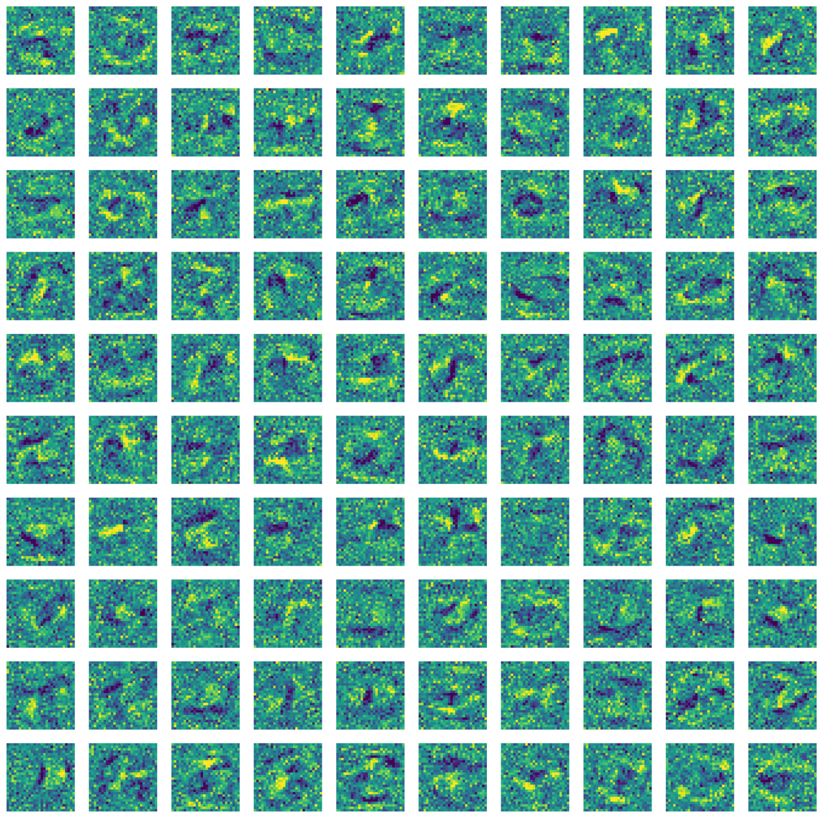
We can tell that they are detecting features of some kind but they are hardly interpretable. Remember they will be weighted and mixed together in the next layer, so the interactions can be very complex.

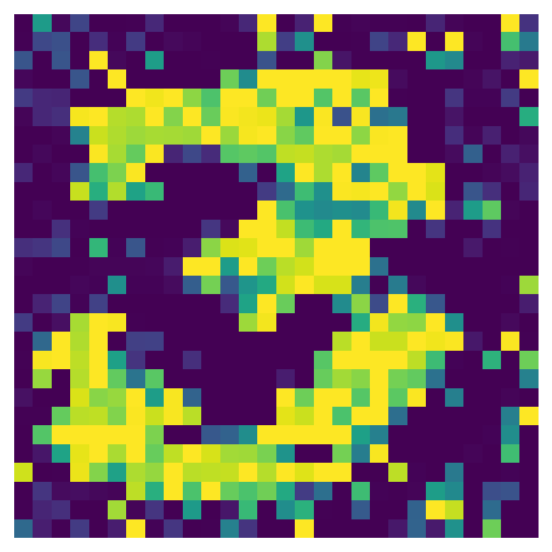
Another way to understand what the network is paying attention to is activation optimisation. Here, using the PyTorch model, we optimise the input to maximise the output probability of the 3,

Future Exploration

• Computational efficiency spin - use a lower level language to try and minimise memory footprint and / or runtime for training and inference.
• Animate 3 appearing in activation optimisation image during training